Earth Temperature Anomalies are Not 2nd Degree Polynomial Behaviors Joel M Williams

Earth Temperature Anomalies
are Not
2nd Degree Polynomial Behaviors

Joel M Williams ©2015

For a free pdf file click here

Abstract

This article illustrates that, while the rising level of CO₂ in the atmosphere from 1900-2015 may fit a 2nd-degree polynomial tightly (R²=0.99+) relative to time (years), the shot-gun-appearing, annual temperatures for the contiguous US for the same period do not. Neither a linear fit (R²=0.23) nor a 2nd-degree polynomial fit (R²=0.27) properly characterizes the annual temperature/time behavior. A running average clearly demonstrates cyclical behavior of the set of annual US temperatures and that these cycles will impinge on the temperature magnitudes expected in the future. The highly alarmist predictions of an upward-turned, 2nd-degree, polynomial into the future are greatly out of sync with these.

With all of the commotion about global warming, I decided to look into the NOAA Drought Index for the Contiguous US for the month of May for the years 1998-2015. I was struck by how extreme the changes were from year-to-year and from region-to-region while watching the video I made. I wondered if these changes corresponded to the average US temperature changes that occurred from year-to-year during the same month. These data are plotted below:

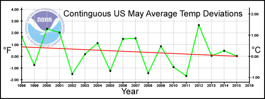
When I added this info to my video, it was apparent that, while Drought Index changes in some regions might correspond to these deviations, the climate changes in the whole contiguous US were too great to be explained by the US average. The exercise did provides some interesting information: 1) the average May temperature in the contiguous US has generally declined during the past 17 years, with 2) year-to-year changes as great as 4.4°F (2.4°C); this while CO₂ level increased slightly. This got me thinking again about the global warming issue as related to the US; the US being a prime driver in global warming alarm and analysis.

The graph on the right shows the annual (June-May, so that the current year could be included) anomaly temperatures for the contiguous US from 1900-2015. 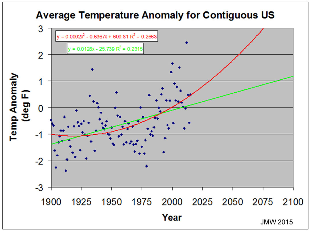The first thing of note is the tremendous scatter from year-to-year! Selective choosing of time ranges can give tremendous differences in analyses. Two regression lines are shown for the entire set. Neither "model" shows that the data are greatly related to the time (years) factor to which CO₂levels can be smoothly related: R² = 0.266 for the 2nd-deg and 0.23 for the linear fit. Within the bounds of the years covered, the two would hardly be deemed different with individual deviations from the "models" reaching ±2°F. The difference between the two "models" is in their prediction of future data! Neither treats the "shotgun" appearing data well, in any case.

Is there a way to reduce the scatter? Yes, one way is to assume that the year-to-year data have some commonality that will be enhanced by a "running" average. The orange line in the figure on the right is for a 5-year running average; a 7-year one is only slightly different. Several things are of note:

1) This data set has two major highs and lows with minor ones in and between each.

2) Neither the linear nor the 2nd-deg regression duplicates the cyclical nature of the running average.

Why would one expect linear and 2nd degree treatments to even be satisfactory for such co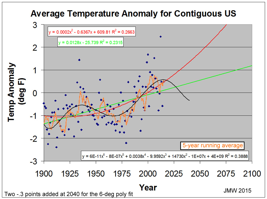mplicated systems, like climate changes, that are surely multidimensional? What is a minimal polynomial equation that can treat the data and reflect the "running average" character? The figure on the right shows the results for a regression of the individual data (not the running average) with a 6th-degree polynomial. R²=0.40. There is still much scatter that is unrelated to this component, however. This model predicts that the "running average" will be making an ~80-year downturn.

Since the major component is rather broad through the main portion of the data, it seems likely that the region near the end of the data set should 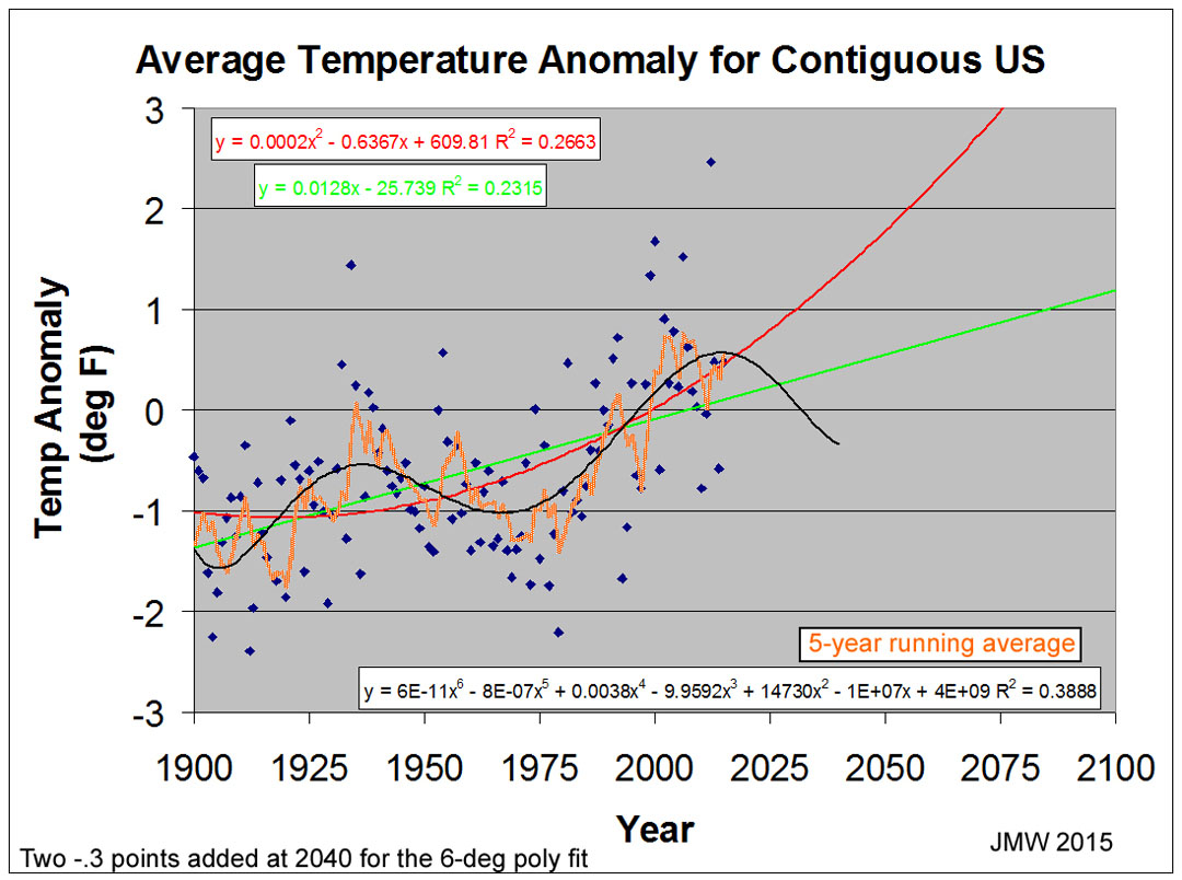not be as narrow as the 6th-deg polynomial indicates. To make the peak broader, two (-0.3) points have been added (at 2040) for the regression in the figure on the right. R²= 0.39. Note that the linear regression lines goes through the inflection points of the 6th degree polynomial regression and, thus, indicates its slope. While it does indicate a positive slope during this time period, it does not necessarily "verify" cause-and-effect due to CO₂ level.

The 6th-degree polynomial indicates that the 5-year running average behavior should be peaking or has. There will be deviations of the running average from this polynomial fit, but they should be small. There will be many extreme deviations of individual (annual) data from the regression in both high AND low directions, however, as the current data indicate "shot-gunny" character due to OTHER factors.

A 2nd degree polynomial fits the growth of singular-component CO₂ in our atmosphere very well: at least, until it levels or falls. The CO₂ regression of th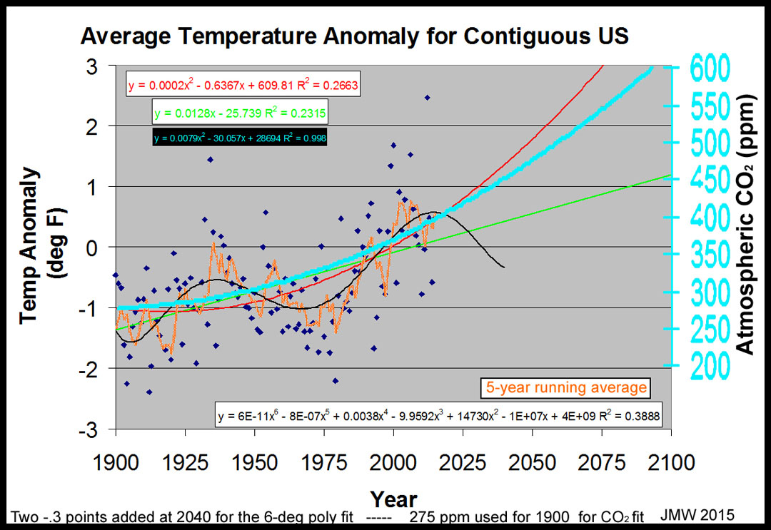e Mauna Loa data for 1959-2014 with a 275ppm point at 1900 (R²=0.99+) is included in the graph on the right. The CO₂ scale is set so that 400ppm is the current value and then touches the linear green line. I believe that some would simply overlay the red line. While 2nd degree polynomial may be fine for CO₂, it is not appropriate for temperature anomalies that are multivariate. A linear regression predicts significant positive anomalies in the future, but it is better than the 2nd degree polynomial regression that goes exponentially upward. The latter will continue to be extremely alarmist, even if future data to the contrary is added. This alarm will continue until enough new data (a century's worth?) is added to cause it to have a parabolic peak. As note before, individual annual points should continue to be widely scattered about the 6th-degree polynomial regression line in the future as they have in the past. The scatter is so great that 60% of the annual temperature data does NOT even conform to this regression! I would guess that there are many cosmic influences that provide significant impact -- some probably even contribute to the linear component! The Vostok Ice Core shows many turns in the earth's global temperature; one with an ~100,000-year cycle.