Using GRASS GIS to analyze cell phone information from mission 080103

With the full benefit of hindsight, I took the information available from mission 080103 to examine how GIS (Geographic Information System) techiniques could be used for planning purposes, had such tools been available to planners.

Tools

I am primarily using the GRASS GIS software, with miscellaneous tools from the GDAL library to process source data such as USGS Digital Elevation Models (DEM) and USGS Digital Raster Graphics (DRG, topo maps). I have a DVD-ROM of all the DEM and DRG files for all of New Mexico. I can legally redistribute that data, or it can be purchased from GeoCommunity.

Information available

Verizon reports that the subject's cell phone was heard by the tower at 222 East Marcy Ave on the northeast side at 8.8 miles.
Verizon reports that the subject's cell phone was also heard by a tower at 1684 Paseo de Las Vistas (35.68876 degrees N by 105.978862 degrees W) at a distance of 10.9 miles, also to the northeast.
Subject claims to be at 11,900 feet reading his barometer watch.
Subjects have been out for several days in wildly variable weather conditions.

Plotting the cell phone data

The primary trick to plotting the cell phone data is getting latitude and longitude coordinates for the two cell towers. Verizon provided one, and I looked up the second using a postal address geocoder and the US Census TIGER/LINE data for Santa Fe County. The Census data is notoriously bad, but gives a reasonable guess at the location of 222 East Marcy Avenue as 35.688295N by 105.934948W. [A few days later I learned of a web site (www.towersource.com), that allows lookups of tower sites, and confirms the coordinates to within a few ten-thousandths of a degree.]

The graphic below shows the data from 222 East Marcy, plotted as an approximate circular arc of radius 8.8 miles, but smeared to assume a +/- 0.2 mile uncertainty in the measurement (just a number obtained through rectal extraction.) The large grey rectangles are the outlines of the Aspen Basin and McClure Reservoir quads, which would be unreadable at this scale. The assumption is a rough beamwidth of 90 degrees centered on a bearing of 45 degrees true.

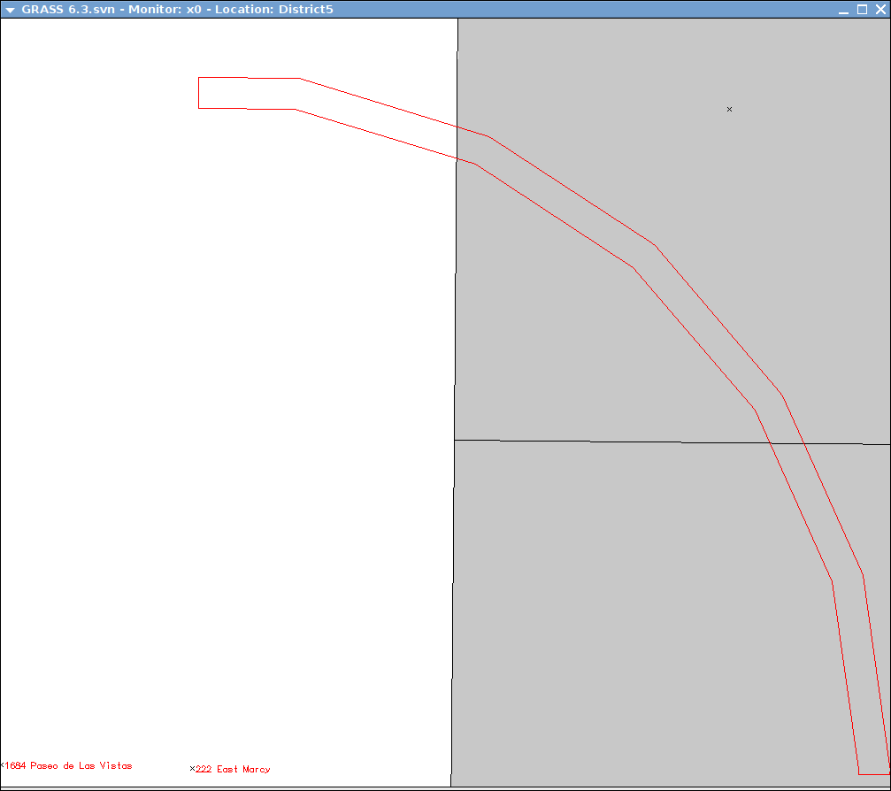
This wedge is the result of a handful of GRASS commands which I have put together in a script to make it easy to do. Basically it boils down to these operations:

form a buffer 8.8 miles around the point 222 East Marcy
Form a ring by buffering 0.2 miles in and out of the circle just obtained.
Form a triangle with a vertex at the center of the circle and the right angles (pointing in the right direction, and with the right angle at the center)
Form the overlap between the ring and the triangle.

The result of those operations is the red area outlined. My script makes this a single operation I call a 'buffer wedge' -- it just does all those steps under the hood.

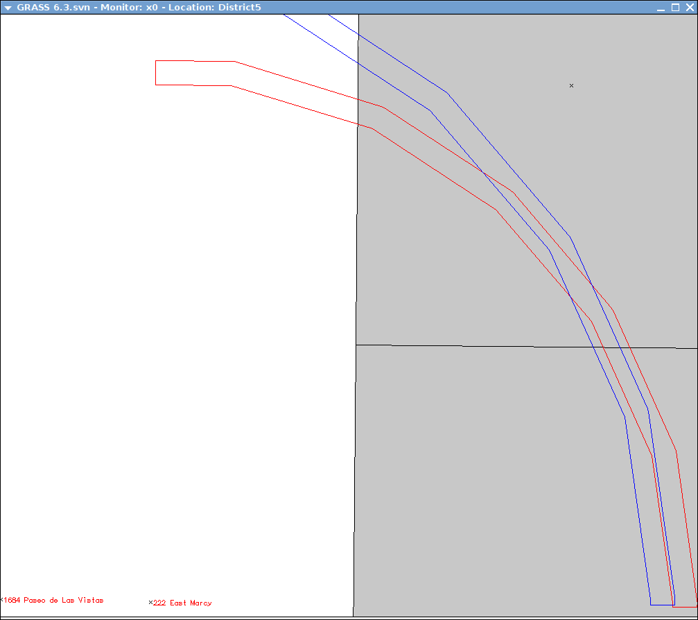
Applying the "buffer wedge" operation to the second cell tower data gives the picture below.

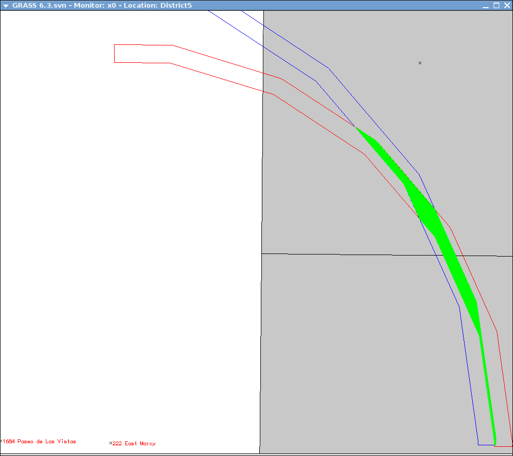
At this point the figure is a little hard to read, so we apply an overlap operator using the GRASS function "v.overlay." The figure below shows in green the area covered by both of the "wedges" of cell phone uncertainty. Using two simple GRASS functions ('v.db.addcol' and 'v.to.db') we can compute the area of the overlap, which turns out to be a bit less than 1.3 square miles.

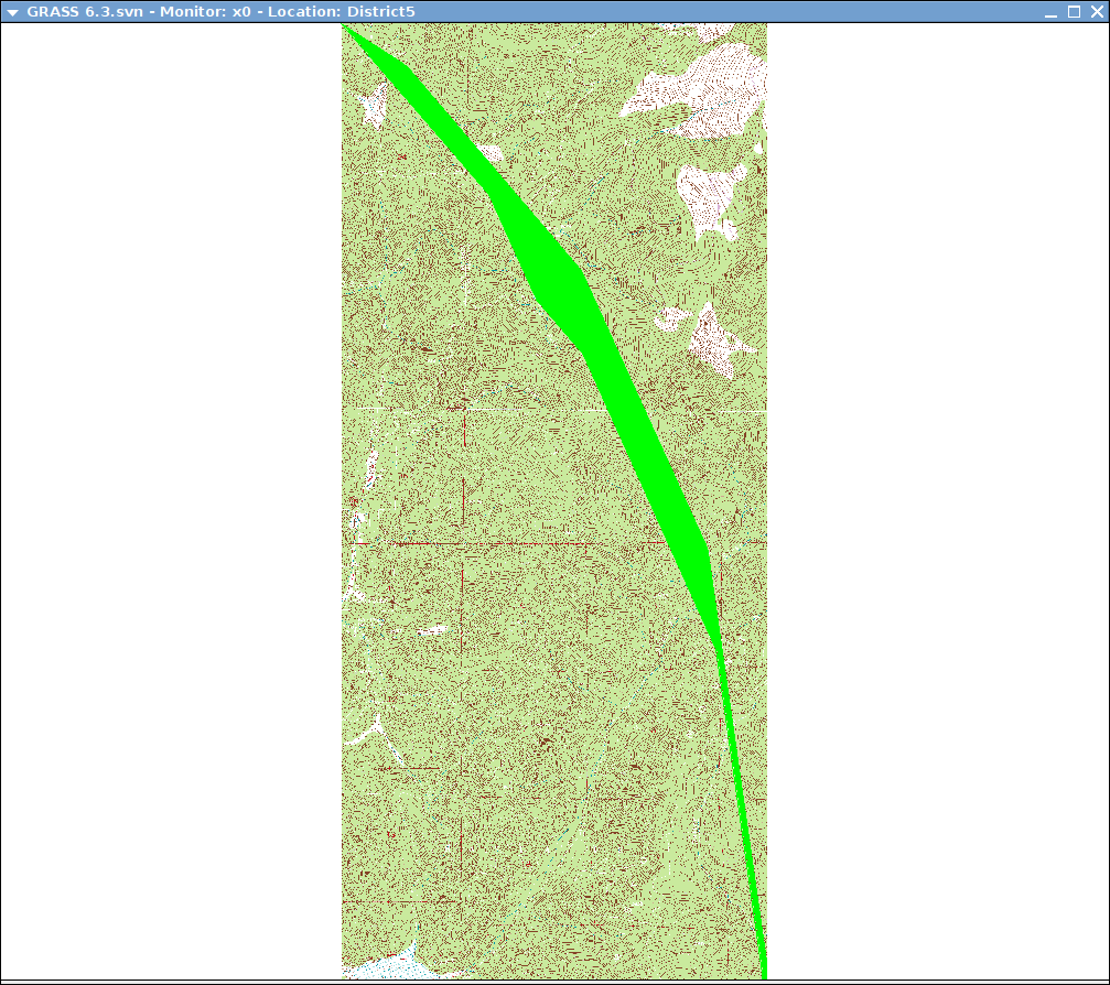
At this point, we don't need the wedges anymore, so I redraw the screen without them, using only the overlap polygon. This time I draw them over the two topo maps, but we're still zoomed out too far to see any real detail.

The final piece of the puzzle is the subject's claim that his watch says he's at 11,900 feet. Since the weather has been so variable and he is unlikely to have recalibrated his altimeter after being caught in the storm, let's just say that means his altitude is above 11,000 feet. We can use the GRASS functions "v.to.rast" and "r.mapcalc" to compute all the points in the map that meet all the following criteria:

Are inside the overlap region, meaning they're in points that might correspond to areas that could have produced the cell phone information we have. (we do this by rasterizing the vector overlap with v.to.rast to make a grid of pixels that are 1 inside the area and null outside.)
Are above 11,000 feet

We combine these two requirements with a messy, but relatively straightforward set of instructions to r.mapcalc that pretty much correspond to the words written in the list above. This produces us a raster with 1 only in the places where both criteria are met, and null outside.

This turns out to be a very restrictive pair of criteria, the results of which are shown by the magenta area in the figure below:

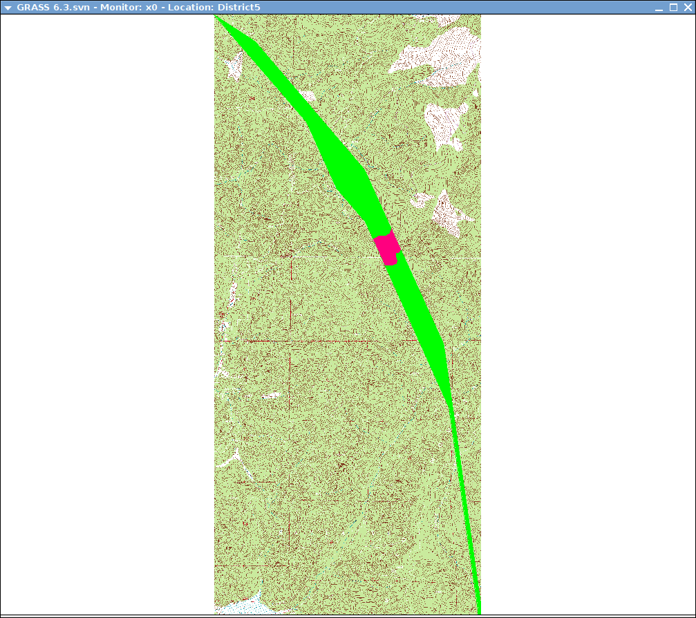
This raster can be turned back into a vector with one command, too, r.to.vect. The result is a search area we can plot on a map as a boundary. We can also use the "v.db.addcol" and "v.to.db" functions again to compute its area, which turns out to be 0.08 square miles.

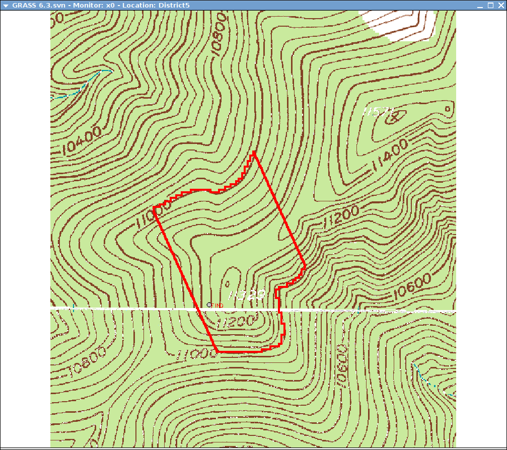
Note that the actual location of the subject is plotted on this final image.

The entire thing can then be packaged up into a PDF map for printing, although making this pretty is more time consuming than it should be. The GRASS function used is ps.map, and one constructs an input file for it such as this one, which produced a postscript file to be converted to this PDF file.

Further refinements possible

One thing I did not do is to compute from the cell phone tower locations the points on the mountain that have line-of-sight to the towers. The very fact that the towers heard the call at all could severely reduce the probability that the subjects were calling from a location below the horizon as viewed from the top of the tower. This is also a relatively simple calculation in GRASS which has a function called "r.los" that will compute all the locations that have line-of-sight to a chosen location, given a digital elevation model and the height of the observer above the ground at that location. (This is also useful for producing truncated maps of what can be seen when standing at a given location.)

Conclusion

With a little preparation, it is well within the capabilities of a free GIS tool to combine the information available on mission 080103 to construct a reasonable search area that fits it in an operationally reasonable way. The area it pinpoints is small enough to justify tossing a small number of resources there even if "common knowledge" overwhemlingly pushes the search into what is considered more likely areas.

Obviously, using these tools would require that planning section have access to a technical specialist familiar with them. But these tools are freely available and far more powerful than the commercial "mapping programs" that are common in SAR base. I highly recommend that SAR managers cultivate a pool of GIS-savvy volunteers to assist with planning.