Click image for free 18Mb pdf of this "out-of-print" book	This article and others are included in the 18 chapters of "Rethinking the Atom" a 164 page paperback compilation of articles by JMW $19.95 US list at Amazon Click here  for Amazon.com	Click image for free 22Mb pdf of the book

The Spherical Cloud Model of Electron Orbitals

Orbitals are intended to provide a handle on how electrons might be arranged around a nucleus. The data presented by Stodolna, et al[1] using a ‘quantum microscope’ technique indicate that electrons are not randomly dispersed.  They suggest that their results might indicate “circular or spherical” orbitals for the hydrogen atom. While one might wonder about some indu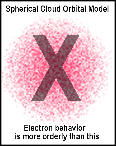ced artifacts, it is clear from their images that hydrogen orbitals are fairly well defined. “Dot-matrix” cloud representations[2] of electron orbitals, as depicted in the figure at the right, and their hybrid mixings are not and are, thus, misleading. Such representations are presumably efforts to convey probability distributions that are based loosely on static (no time factor) continuum calculations. They provide no information about how or why an electron got to a possible location or where it would go next. Speaking of an electron as a cloud and then saying the cloud is densest where that electron can be found is doublespeak!

The ‘quantum microscope’ experimental data, also discussed further below, show that electrons behavior is quite orderly. Indeed, the constancy and sharpness of spectral data have ALWAYS indicated this. It is strange that the electron in a cloud model, which might be in any position, low near the nucleus or far from it, nevertheless jumps in response to the exact same photon into one precisely higher orbital position, regardless of the point from which it jumps. Unless there are significant qualifications to the observed experimental location and spectral data, “electrons-can-be-anywhere-and-everywhere” probability models make no sense! Thus, models such as that depicted in the figure above should be nixed!

Electron Orbitals as Generated by the MCAS Model  

While the authors of the ‘quantum microscope’ data indicated that their results might indicate “circular/spherical” orbitals for the hydrogen atom, the data also supports non-spherical orbital shapes. Actually, the data may only represent the summation of the outer (zenith and nadir) limits of electron movement at each energy level.[3] These are the points of zero movement from the nucleus where the electron is most likely to be observed. Indeed, electrons are observed as particles whose “roundness” and dipole character are now being sought![4] Could they actually be too pudgy to be quantum changelings? “Electron-spin predestined the predominant singular twist of natural molecules (e.g., DNA). With a singular spin, electrons flow chirally around nuclei. Thus, electronic orbitals possess built-in chirality. Atoms of the universe were the first to have a one-way traffic system.”[5] Orbitals should be considered as defining where electrons travel alone on beaten “paths”, ruts, tubular conduit worm-holes or as in sync groups possibly like “necklace” beads on an orbital “string” wave. While it may be easier to draw orbitals with conical lobes, the actual paths may be more like twisted paddles. Spin-pairing occurs in the MCAS model with electrons flow in opposing orbitals in contrast to the current electron-spin reversal requirement.

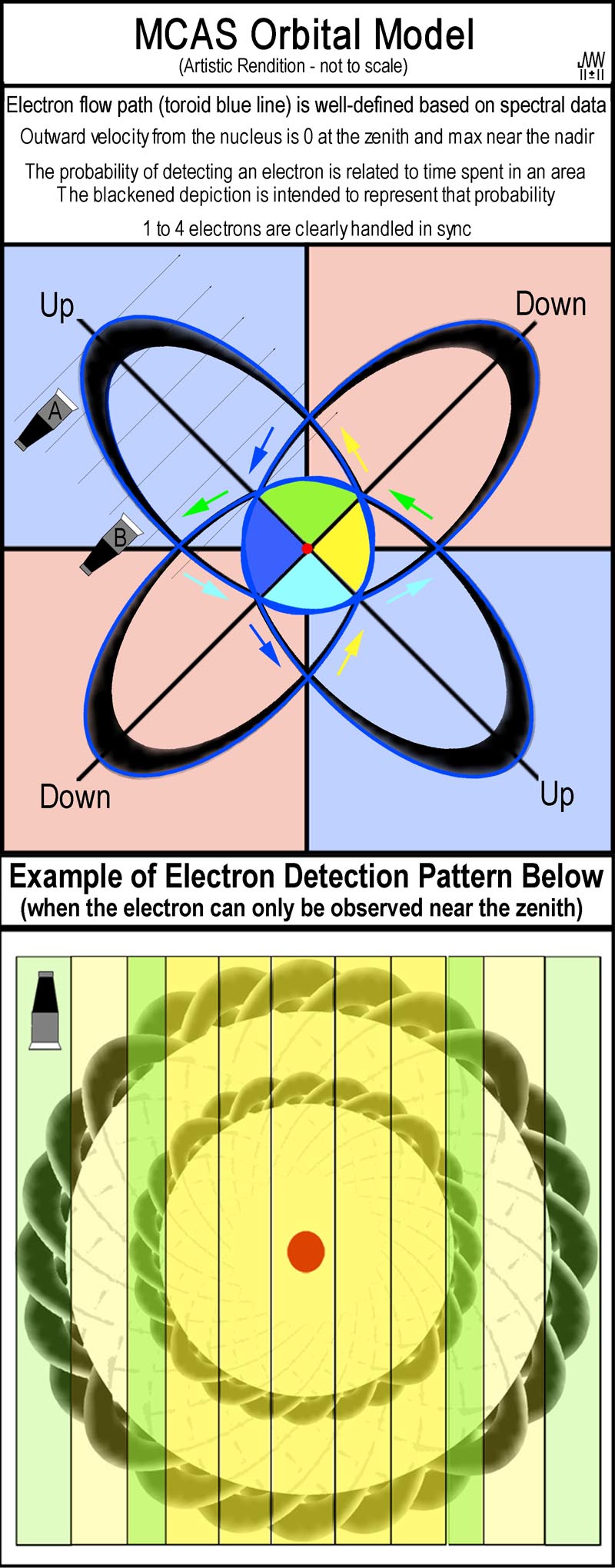The following discussion demonstrates how electrons will be observed per the MCAS model. The figure at the right is a flattened MC tetrahedral orbital which the model would use for a hydrogen atom’s simplest levels. The depiction is “not to-scale”. The lobes in the blue quadrants were “Up”, while those in the pink quadrants were “Down”. Electron movement will be along very narrow paths as illustrated by the blue-lined hypotrochoid. The lobe dimensions are set by the energy of the electrons and their electrostatic interaction with the nucleus. The extent of the lobes is integer-based (n² = 1, 4, 9, etc); a simple demonstration of why this is so has been presented elsewhere[6]. Black areas inside the blue orbits are included to provide a rough indication of the probability of an electron being observed. At the orbital zenith, the electron is neither moving from nor towards the nucleus. Just before and afterwards, it is also slow in that regard; elsewhere, movement to/from the nucleus is quite rapid. Detecting an electron depends on the observing device’s response time and sensitivity. While detection of an electron may be obtained with “sensor A”, the same setting on “sensor B” (or a single sensor viewing the entirety) may show nothing as an electron speeds past its view. The situation becomes similar to the image in the figure at the lower right when many ‘sightings’ are made and the tetrahedral orbital’s 3D movement is not anchored along with that of the nucleus. The vertical green strips indicate the perpendicular view that shows where the slowest movement to/from the nucleus occurs and is thus the most likely region for success in detecting electrons. The yellow strip areas are relatively similar to one another and provide much less chance of detecting an electron. With sufficient data merging, details become blurred and smooth rings are generated. Experimental electron detections will be for 3D tetrahedral orbitals; for illustrative purposes, the lobes are shown flattened here.

For a hydrogen atom, a single, particulate, electron can ONLY be at one place at any given moment in time.  A second orbital level is shown to illustrate the cumulative effects of data summing. Depending on conditions, inter orbitals, which are of lower energy, could very well have a higher temporal concentration of that electron and thus show up more intense than outer ones.

Conclusion: the probability of an electron being found at a location depends on temporal as well as non-temporal factors, such as electrostatic interactions and energy levels.

The MCAS Model and ‘Quantum Microscope’ Results

In order to evaluate how the MCAS model fits the ‘quantum microscope’ results¹ , the images from that work have been inspected. That work is very elaborate and extensive. Holding the nucleus in a rigid location is quite impressive as is the detection of an electron’s position. In the end, however, the accomplished effort simply provides a collection of singular results: projected 2D locations of the 3D locations of a single electron, in the case of a hydrogen atom, regardless of how the electron got there. Impressive numbers of singular results were required to indicate that the electron spends time in well-defined “orbitals”.

The figure below has been created to interpret the ‘quantum microscope’ results and to relate the MCAS atomic orbital model to them.

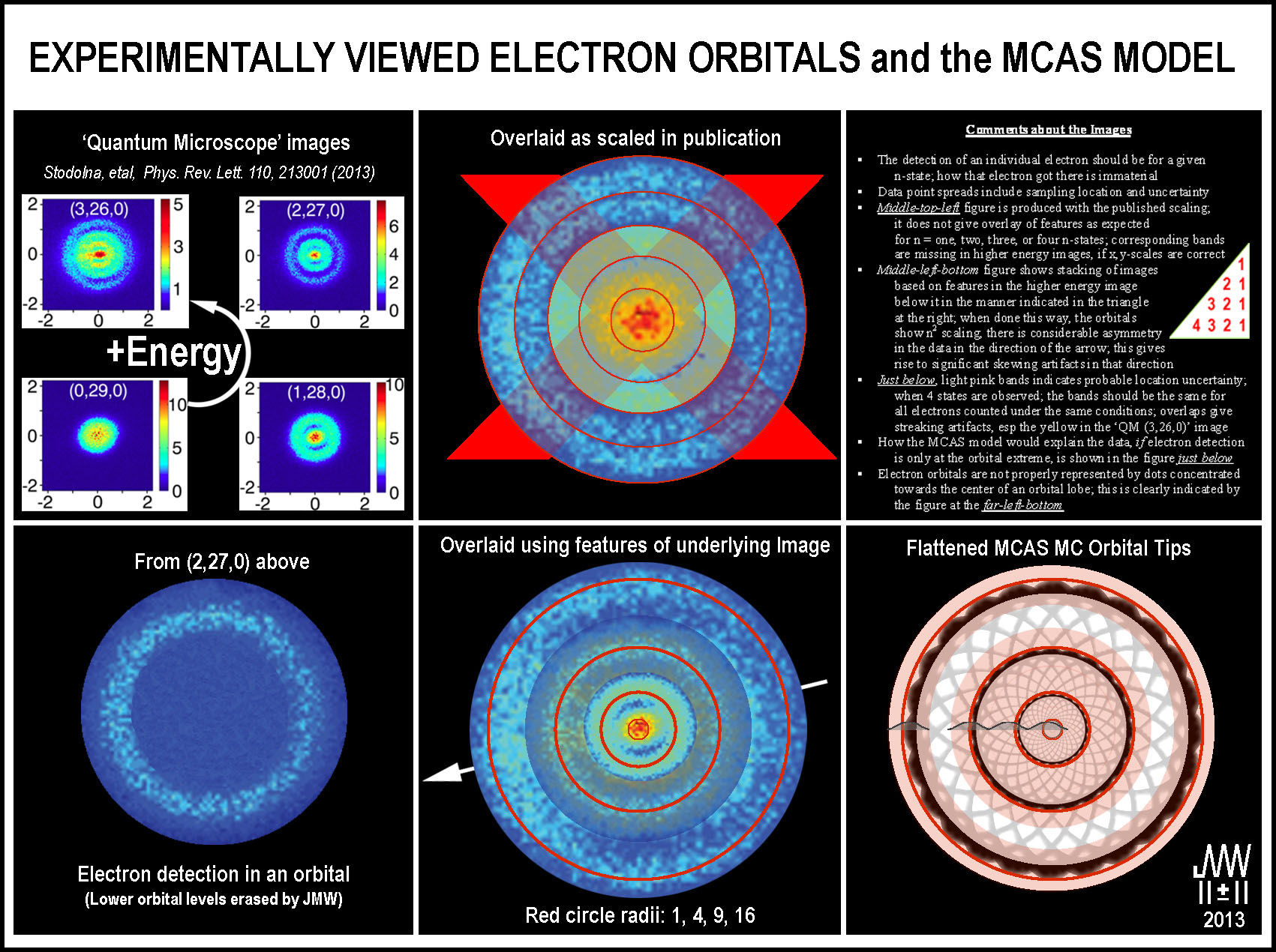
The original images (upper-left set of images) demonstrate cleanly separated, outer regions for the higher activated states. Delving into the inner orbital makeup is a bit difficult when the images are apart. To address this problem, the images, which were indicated in the published work to have the same scale, were stacked with the highest energy image at the bottom (upper-middle image). The outer region of each lower energy image was removed in order not to obscure that portion of the image below. Since the second lowest energy image indicated a tight center, that center was copied and placed on the top. Alternating rings would have to be missing in several of the published images, if the individual x-y scales are correct. Also, some image details, esp. those of the middle two energy level images, do not overlay. This overlay from the publication’s indicated scaling is inconsistent and therefore has been “X’d” out.

The published images are stacked differently in the bottom-middle image. Each lower energy image is scaled to the inner structure of the higher energy one placed just below in the manner indicated in the triangle in the upper-right image. Again, the outer portion of the next upper image is removed to show the outer region of the image below. Images higher in the stack have also been made more transparent to show some of the lower image’s details. While the rings are nearly circular, they are not uniform. An obvious bias (asymmetry in the detection or detector array?) in the populations is indicated by the arrow. This bias is likely a systematic issue in the data collection as it appears in all of images. The spread in the rings is likely from uncertainties in both actual electron locations and experimental error. Together, they will produce the artifacts that prevent the “dark blue” circular regions that separate the lower energy orbitals from being complete and the non-circular skewing in the ‘QM (0,29,0)’ image. More about this is discussed below.

The PhysRevLett article indicates that only four levels are present and that is clearly evident in the bottom-middle image. It is also clear that the levels scale closely to n² = 1², 2², 3², and 4² (see the red circles in the bottom-middle image) when stacked in this manner.

There is considerable asymmetry in the data in the direction of the arrow. This gives rise to significant skewing artifacts in that direction. The light pink circular bands in the lower-right image indicate the possible uncertainty in the characterization of the highest energy orbital of the ‘QM (3,26,0)’ image. It would be the same for all of the orbitals measured under the same conditions. (The second highest energy image (‘QM (2,27,0)’) appears to have a bit less uncertainty which would explain why it is sharper and more widely shown.) The uncertainty bands overlap for the lowest 3 energy orbital states in the ‘QM (3,26,0)’ image; this leads to streaking artifacts, notably, the yellow ones.  

How the MCAS model would explain the data, if electron detection is only at the orbital extreme, is shown in the lower-right-image. The tip portions of the flattened MC-orbitals are placed at the mid-region of the various energy rings. This indicates zero movement towards or from the nucleus. While the electron will move through 3D-space in its journey to and from the nucleus, it is at these zeniths that the electron will most readily be detected. The probability of locating an electron has a time factor as well as the normal electrostatic ones that are typically considered.

The lower-left image shows an experimentally observed orbital – the outer orbital of the ‘QM (2,27,0)’ image – wherein the lower energy orbitals have been erased for clarity. This image clearly demonstrates that electron orbitals are not properly represented by dots concentrated towards the center of an orbital lobe. Dot representations are even more misleading when the lobes are not even nucleus-centered! One should also seriously question the imagery of molecular bonds as “capsules” whose space is filled with dots of ‘electrostatically non-repelling, spin-paired, electrons’.

REFERENCES